42 align data labels excel chart
5 New Charts to Visually Display Data in Excel 2019 - dummies Select the data and labels and then click Insert → Maps → Filled Map. Wait a few seconds for the map to load. Resize and format as desired. For example, you could apply one of the chart styles from the Chart Tools Design tab. To add data labels to the chart, choose Chart Tools Design → Add Chart Element → Data Labels → Show. Controlling Chart Gridlines (Microsoft Excel) Select the chart by clicking on it. You should see selection handles appear around the outside of the chart. Make sure that the Layout tab of the ribbon is displayed. (This tab is only visible when you've selected the chart in step 1.) Click the Gridlines tool in the Axes group. You'll see a drop-down menu appear with various options.
› custom-data-labels-in-xImprove your X Y Scatter Chart with custom data labels May 06, 2021 · Thank you for your Excel 2010 workaround for custom data labels in XY scatter charts. It basically works for me until I insert a new row in the worksheet associated with the chart. Doing so breaks the absolute references to data labels after the inserted row and Excel won't let me change the data labels to relative references.

Align data labels excel chart
› excel-chart-verticalExcel Chart Vertical Axis Text Labels - My Online Training Hub Apr 14, 2015 · So all we need to do is get that bar chart into our line chart, align the labels to the line chart and then hide the bars. We’ll do this with a dummy series: Copy cells G4:H10 (note row 5 is intentionally blank) > CTRL+C to copy the cells > select the chart > CTRL+V to paste the dummy data into the chart. › data-definition-excel-3123415Excel Spreadsheet Data Types - Lifewire Feb 07, 2020 · Text data, also called labels, is used for worksheet headings and names that identify columns of data. Text data can contain letters, numbers, and special characters such as ! or &. By default, text data is left-aligned in a cell. Number data, also called values, is used in calculations. By default, numbers are right-aligned in a cell. Format Chart Axis in Excel - Axis Options The Next option is to adjust the labels on the chart. Labels are nothing but the axis values. We can change the position of axis values relative to the position of the axis line. For now, we are setting the label's position to high. Axis Options : Number Format
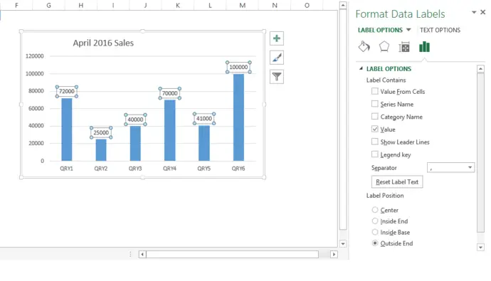
Align data labels excel chart. peltiertech.com › text-labels-on-horizontal-axis-in-eText Labels on a Horizontal Bar Chart in Excel - Peltier Tech Dec 21, 2010 · In Excel 2003 the chart has a Ratings labels at the top of the chart, because it has secondary horizontal axis. Excel 2007 has no Ratings labels or secondary horizontal axis, so we have to add the axis by hand. On the Excel 2007 Chart Tools > Layout tab, click Axes, then Secondary Horizontal Axis, then Show Left to Right Axis. DataLabel.VerticalAlignment property (Excel) | Microsoft Docs Syntax Remarks Returns or sets a Variant value that represents the vertical alignment of the specified object. Syntax expression. VerticalAlignment expression A variable that represents a DataLabel object. Remarks The value of this property can be set to one of the XlVAlign constants. Support and feedback Alignment of Chart Line - Microsoft Tech Community Alignment of Chart Line. Is it possible to move a line in a chart in Excel? I'm trying to get the line to start on the left side of a column rather than starting in the center but I can't find a way to do that. Second option would just be to draw a line, but I figured there had to be a way to adjust the position. Labels: How to format bar charts in Excel - storytelling with data Click on any data label to highlight them all, then right-click and choose Format Data Labels: 4. In the Format Data Labels menu, select Label Options, and in the Label Positions section, choose Inside End. (While you're at it, in the Label Contains section, uncheck "Show Leader Lines.". These are almost never necessary.)
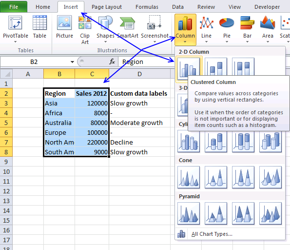
Tree Maps Data Labels and Tables Formatting/Sorting Errors after ... Tree Maps Data Labels and Tables Formatting/Sorting Errors after Windows 11. My Tree Map in Excel and Powerpoint after the Windows 11 update does not order my tables from smallest/largest value correctly, nor allow me to right-align my data labels, nor does it spell out the data label name. Custom Excel number format - Ablebits.com A usual way to change alignment in Excel is using the Alignment tab on the ribbon. However, you can "hardcode" cell alignment in a custom number format if needed. ... Is it possible to display a percentage value without the percentage sign using custom number formatting? I want the chart labels for each data point to be displayed without ... How to Create and Customize a Treemap Chart in Microsoft Excel Either right-click the chart and pick "Format Chart Area" or double-click the chart to open the sidebar. On Windows, you'll see two handy buttons on the right of your chart when you select it. With these, you can add, remove, and reposition Chart Elements. And you can pick a style or color scheme with the Chart Styles button. How to Make a Pie Chart in Excel & Add Rich Data Labels to The Chart! Creating and formatting the Pie Chart. 1) Select the data. 2) Go to Insert> Charts> click on the drop-down arrow next to Pie Chart and under 2-D Pie, select the Pie Chart, shown below. 3) Chang the chart title to Breakdown of Errors Made During the Match, by clicking on it and typing the new title.
How to Overlay Charts in Microsoft Excel - How-To Geek In the Change Chart Type window, select Combo on the left and Custom Combination on the right. Create your chart: If you don't have a chart set up yet, select your data and go to the Insert tab. In the Charts section of the ribbon, click the drop-down arrow for Insert Combo Chart and select "Create Custom Combo Chart." Set Up the Combo Chart Pivot chart X axis labels not aligned to the ... - Excel Help Forum 3) Find the "Series Overlap" setting and change it to "full overlap" or "+100%" or whatever the equivalent is in your version of Excel. I will see if someone more familiar with the O365 UI can provide more details on where and how to find these options. Register To Reply 08-12-2021, 02:19 PM #5 Jigneshbharati Registered User Join Date 12-02-2020 peltiertech.com › excel-column-Excel Column Chart with Primary and Secondary Axes - Peltier ... Oct 28, 2013 · The second chart shows the plotted data for the X axis (column B) and data for the the two secondary series (blank and secondary, in columns E & F). I’ve added data labels above the bars with the series names, so you can see where the zero-height Blank bars are. The blanks in the first chart align with the bars in the second, and vice versa. How to Change the X-Axis in Excel - Alphr Open the Excel file with the chart you want to adjust. Right-click the X-axis in the chart you want to change. That will allow you to edit the X-axis specifically. Then, click on Select Data. Next ...
Custom data labels in a chart | Get Digital Help - Microsoft Excel resource
How to Add Labels to Scatterplot Points in Excel - Statology Step 3: Add Labels to Points. Next, click anywhere on the chart until a green plus (+) sign appears in the top right corner. Then click Data Labels, then click More Options…. In the Format Data Labels window that appears on the right of the screen, uncheck the box next to Y Value and check the box next to Value From Cells.
SSRS Charts with Data Tables (Excel Style) | Some Random Thoughts
Chart control not showing all points' labels on x-axis where pointNames is a string array and value is an int. The chart displays correctly, but only some of the points' names show. Here are all the series properties I set: currentSeries.ChartType = SeriesChartType.Column; currentSeries [ "PointWidth"] = pointWidth; currentSeries.IsValueShownAsLabel = true ; currentSeries [ "BarLabelStyle ...
PrimeNg Chart, display labels on data elements in graph. | by Alok Vishwakarma | Medium
› charts › variance-clusteredActual vs Budget or Target Chart in Excel - Variance on ... Aug 19, 2013 · Set Data Labels to Cell Values Screenshot Excel 2003-2010. The nice part about either of these methods is that the data labels are linked to the values in the cells. If your numbers change or you update the data, the labels will automatically be refreshed and display the correct results. Please let me know if you have any questions.

Excel Variance Charts: Making Awesome Actual vs Target Or Budget Graphs - How To ...
Date Axis in Excel Chart is wrong • AuditExcel.co.za In order to do this you just need to force the horizontal axis to treat the values as text by. right clicking on the horizontal axis, choose Format Axis. Change Axis Type to be Text. Note that you immediately lose the scaling options and the date scale puts in exactly what is in the data, onto the horizontal axis.

Directly Labeling Excel Charts | PolicyViz
Excel Waterfall Chart: How to Create One That Doesn't Suck If your data has a different number of categories, you have to modify the template, which again requires additional work. Ideally, you would create a waterfall chart the same way as any other Excel chart: (1) click inside the data table, (2) click in the ribbon on the chart you want to insert. ... in Excel 2016

Excel Vba Chart Label Alignment - chart elements in excel vba part 2 series data labels แทงฟรี ...
Two-Level Axis Labels (Microsoft Excel) - ExcelTips (ribbon) Place your row labels into column A, beginning at cell A3. Place your data into the table, beginning at cell B3. With your table completed, you are ready to create the chart. Just select your data table, including all the headings in the first two rows, then create your table.

After formatting each label, you can delete the legend and style the gridlines, tick marks, etc ...
› shortcuts › align-centerExcel Align Shortcuts - Left, Center, and Right - Automate Excel Align Center This Excel Shortcut applies Align Center Formatting PC Shorcut:ALT>H>A>C Mac Shorcut:⌘+E Remember This Shortcut: PC: Alt is the command to activate the Ribbon shortcuts. H for Home, A for Align, C for Center Align Left This Excel Shortcut applies Align Left Formatting. PC Shorcut:ALT>H>A>L Mac Shorcut:⌘+L Remember This Shortcut: PC: Alt is the…

Right-aligning Y-axis labels on a stacked bar chart : excel
DataLabel.HorizontalAlignment property (Excel) | Microsoft Docs In this article. Returns or sets a Variant value that represents the horizontal alignment for the specified object.. Syntax. expression.HorizontalAlignment. expression A variable that represents a DataLabel object.. Remarks. The value of this property can be set to one of the XlHAlign constants.. Some of these constants may not be available to you, depending on the language support (U.S ...
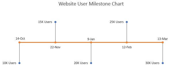
How to Create Milestone Chart in Excel
How To Tally in Excel by Converting a Bar Graph to a Tally Graph To do so, double click on your chart to open a window on the side of your Excel spreadsheet with the title "Format Chart Area." Click "Chart Options" and select "Vertical (Category) Axis" from the drop-down menu. Then, click on the "Axis Options" icon at the right of the icon option list and click "Axis Options."

How to Make a Pie Chart in Excel & Add Rich Data Labels to The Chart!
spreadsheetplanet.com › add-gridlines-in-chart-excelHow to Add Gridlines in a Chart in Excel? 2 Easy Ways! So, a second way to add and format gridlines is to use the Design tab from the Chart Tools. Here’s how: Click on your chart. You should see the Chart Tools menu appear in the main menu. Select the Design tab from the Chart Tools menu. Click on ‘Add Chart Element’ (under the ‘Chart Layouts’ group).
Formula Friday - Using Formulas To Add Custom Data Labels To Your Excel Chart - How To Excel At ...
How to Change the Y Axis in Excel - Alphr Click the dropdown next to "Display Units," then make your selection such as "millions" or "hundreds." To label the displayed units, go to the "Axis Options -> Display units" section. Add a...
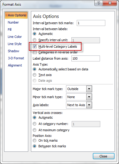
Fixing Your Excel Chart When the Multi-Level Category Label Option is Missing. - Excel Dashboard ...
Clustered Column and Line Combination Chart - Peltier Tech Excel's column and bar charts use two parameters, Gap Width and Overlap, to control how columns and bars are distributed within their categories. Gap Width is the space between bars in adjacent categories, given as a percentage of the width of a column in the chart. The default is 219%, which means the gap is 2.19 times the width of a column.
Creating a chart with dynamic labels - Microsoft Excel 2016
Pie Chart Best Fit Labels Overlapping - VBA Fix - Microsoft Tech Community I created attached Pie chart in Excel with 31 points and all labels are readable and perfectly placed. It is created from few clicks without VBA using data visualization tool in Excel. Data Visualization Tool For Excel Data Visualization Tool For Google Sheets It has auto cluttering effect to adjust according to your data size.

Excel Charts | How to Create a Chart in Excel | MS Excel in Hindi
How to Print Labels from Excel - Lifewire To label legends in Excel, select a blank area of the chart. In the upper-right, select the Plus ( +) > check the Legend checkbox. Then, select the cell containing the legend and enter a new name. How do I label a series in Excel? To label a series in Excel, right-click the chart with data series > Select Data.

Make Excel charts primary and secondary axis the same scale • AuditExcel.co.za
Make Excel charts primary and secondary axis the same scale First create 2 new columns and call then Primary and Secondary Scale. In the first cell create a MIN function that looks at ALL the original data points and finds the smallest number. In the last cell do the same but this time a MAX to find the biggest number out of all the data points. In E8 and E34 just equals to the adjacent cells.

How to add data labels from different column in an Excel chart?
Custom Chart Data Labels In Excel With Formulas Select the chart label you want to change. In the formula-bar hit = (equals), select the cell reference containing your chart label's data. In this case, the first label is in cell E2. Finally, repeat for all your chart laebls. If you are looking for a way to add custom data labels on your Excel chart, then this blog post is perfect for you.
Move and Align Chart Titles, Labels, Legends with the Arrow Keys - Excel Campus
How to format Excel so that a data series is highlighted differently ... 5. To vary the line style, highlight the data point of interest the same way you did earlier in Step 1. Right-click and choose Format Data Point. 6. In the Fill & Line tab again, instead of clicking on Marker, click into the Line menu, where you can adjust the various settings of the line immediately preceding the data point.

How to move chart X axis below negative values/zero/bottom in Excel?
› excel › how-to-add-total-dataHow to Add Total Data Labels to the Excel Stacked Bar Chart Apr 03, 2013 · Step 4: Right click your new line chart and select “Add Data Labels” Step 5: Right click your new data labels and format them so that their label position is “Above”; also make the labels bold and increase the font size. Step 6: Right click the line, select “Format Data Series”; in the Line Color menu, select “No line”
Post a Comment for "42 align data labels excel chart"