40 edit labels in excel chart

› dynamically-labelDynamically Label Excel Chart Series Lines • My Online ... Sep 26, 2017 · To modify the axis so the Year and Month labels are nested; right-click the chart > Select Data > Edit the Horizontal (category) Axis Labels > change the ‘Axis label range’ to include column A. Step 2: Clever Formula. The Label Series Data contains a formula that only returns the value for the last row of data. Adjusting the Order of Items in a Chart Legend (Microsoft Excel) You can select one of the entries and use the up and down arrows (just to the right of the Remove button) to adjust the order in which the entries are plotted. When you click OK, the chart is replotted and the legend updated to reflect the plotting order. ExcelTips is your source for cost-effective Microsoft Excel training.

How to Add a Secondary Axis to Charts in Microsoft Excel? Adding a Secondary Axis in Excel - Step-by-Step Guide. 1. Download the sample US quarterly GDP data here. …. 2. Open the file in Excel, and get the quarterly GDP growth by dividing the first difference of quarterly GDP with the previous quarter's GDP. 3. Select the GDP column (second column) and create a line chart.

Edit labels in excel chart

How to Create a Dynamic Chart Title in Excel Steps to Create Dynamic Chart Title in Excel Converting a normal chart title into a dynamic one is simple. But before that, you need a cell which you can link with the title. Here are the steps: Select chart title in your chart. Go to the formula bar and type =. Select the cell which you want to link with chart title. Hit enter. A Beginner's Guide on How to Plot a Graph in Excel How to Plot a Graph in Excel (step-by-step Instruction) STEP 1: Specify the units of measurement. STEP 2: Enter your data into Excel sheet. STEP 3: Make a data table. STEP 4: Choose the best graph and chart options that suit your operation. STEP 5: Select your data table and insert your desired graph. How to add a single vertical bar to a Microsoft Excel line chart In the Format Axis pane, change the Maximum Bounds value to 1,800,000. Next, expand the Labels heading in the Tick Marks section and choose None from the Label Position dropdown shown in Figure H....

Edit labels in excel chart. Gridlines in Excel - Overview, How To Remove, How to Change Color In the Excel Options dialog box that opens, click Advanced on the left panel. Scroll down to Display Options section. At the bottom of this section, use the Gridline color box to expand the dropdown list. Choose your preferred gridline color and then click OK at the bottom to close the Options dialog box. Step-by-Step Guide on How to Make a Chart in Excel (And Tips) Then click on the "Chart Title" label at the top of your chart to edit the chart name to reflect the project's title. You may also use the "Font Type" and "Font Size" features to emphasize the title and differentiate it from other parts of the chart. 8. Save the chart After creating the chart, the next step is to save it. How To Show Two Sets of Data on One Graph in Excel Choose "All Charts" and click "Combo" as the chart type From the options in the "Recommended Charts" section, select "All Charts" and when the new dialog box appears, choose "Combo" as the chart type. These let Excel know you want to work with multiple data sets before you even edit the graph. linkedin-skill-assessments-quizzes/microsoft-excel-quiz.md at ... - GitHub In the cells group on the Home tab, click Format > Format Cells. Then click the Alignment tab and select Right Indent. Click the Decrease Decimal button once. Q13. Which formula is NOT equivalent to all of the others? =A3+A4+A5+A6 =SUM (A3:A6) =SUM (A3,A6) =SUM (A3,A4,A5,A6) Q14.

› 509290 › how-to-use-cell-valuesHow to Use Cell Values for Excel Chart Labels Mar 12, 2020 · If these cell values change, then the chart labels will automatically update. Link a Chart Title to a Cell Value. In addition to the data labels, we want to link the chart title to a cell value to get something more creative and dynamic. We will begin by creating a useful chart title in a cell. We want to show the total sales in the chart title. support.microsoft.com › en-us › officeEdit titles or data labels in a chart - support.microsoft.com If your chart contains chart titles (ie. the name of the chart) or axis titles (the titles shown on the x, y or z axis of a chart) and data labels (which provide further detail on a particular data point on the chart), you can edit those titles and labels. You can also edit titles and labels that are independent of your worksheet data, do so ... Publish and apply retention labels - Microsoft Purview (compliance) Applying retention labels in Outlook. To label an item in the Outlook desktop client, select the item. On the Home tab on the ribbon, click Assign Policy, and then choose the retention label. You can also right-click an item, click Assign Policy in the context menu, and then choose the retention label. How do I add additional labels to an excel chart? - Stack Overflow I've got a chart in excel and I'd like to add additional labels to it. In the below example I want to add "Inadequate" next to the 34s, "Inconsistent" next to the 42 and so on. Ideally, I'd like to be able to tweek how the floating text looks. I've tried adding an extra row in my data below, but it just messes up the whole chart or isn't useful.

superuser.com › questions › 1484623Can't edit horizontal (catgegory) axis labels in excel Sep 20, 2019 · I'm using Excel 2013. Like in the question above, when I chose Select Data from the chart's right-click menu, I could not edit the horizontal axis labels! I got around it by first creating a 2-D column plot with my data. Next, from the chart's right-click menu: Change Chart Type. I changed it to line (or whatever you want). Learn to Use a Label Creator Add-in Extension in Dynamics 365 for ... The OnClick method is called when the user clicks on our menu. We will modify this method to convert the text contained in the Label property to an actual label. To do this, create regular expression to distinguish between a label identifier and a normal string. › make-labels-with-excel-4157653How to Print Labels From Excel - Lifewire Apr 05, 2022 · To label chart axes in Excel, select a blank area of the chart, then select the Plus (+) in the upper-right. Check the Axis title box, select the right arrow beside it, then choose an axis to label. Two level axis in Excel chart not showing • AuditExcel.co.za Right clicking on the horizontal access and choosing Format Axis Choose the Axis options (little column chart symbol) Click on the Labels dropdown Change the 'Specify Interval Unit' to 1 If you want you can make it look neater by ticking the Multi Level Category Labels

What to do with Excel 2016's new chart styles: Treemap, Sunburst, and Box & Whisker | PCWorld

Create and Modify a Chart Programmatically - DevExpress Refer to the following section for information on how to organize data in the source range to create a specific chart: Arrange Worksheet Data to Create a Chart. C#. VB.NET. // Create a column chart using a cell range as a data source. Chart chart = worksheet.Charts.Add (ChartType.ColumnClustered, worksheet ["B2:F6"]);

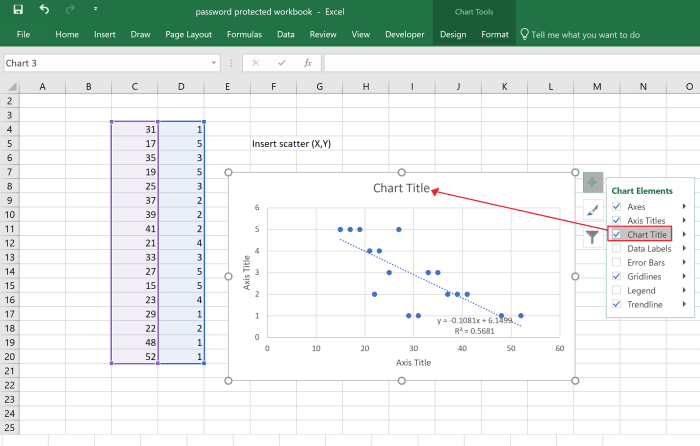
How to Create a Scatter Plot in Excel - TurboFuture - Technology

50 Excel Shortcuts That You Should Know in 2022 - Simplilearn You can see below we have hidden the Chairs, Art, and Label subcategories. Fig: Pivot chart on the same sheet Have a look at the video below that explains worksheet related shortcuts, row and column shortcuts, and pivot table shortcut keys. Conclusion Excel shortcut keys will indeed help you build your reports and analysis faster and better.

Format Number Options for Chart Data Labels in PowerPoint 2011 for Mac

› documents › excelHow to rotate axis labels in chart in Excel? - ExtendOffice Rotate axis labels in Excel 2007/2010. 1. Right click at the axis you want to rotate its labels, select Format Axis from the context menu. See screenshot: 2. In the Format Axis dialog, click Alignment tab and go to the Text Layout section to select the direction you need from the list box of Text direction. See screenshot: 3.

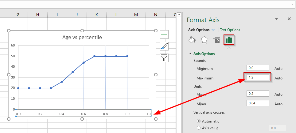
MS Excel - Limit x-axis boundary in Chart | OpenWritings.net

How to Change Date Format in Pivot Table in Excel - ExcelDemy Firstly, click on the Group Selection option in the PivotTable Analyze tab while keeping the cursor over a cell of the Order Date (Row Labels). Secondly, you'll get the following dialog box namely Grouping. And choose Years from the options. Finally, you'll get the sum of sales based on the years instead of the dates. 3.2.

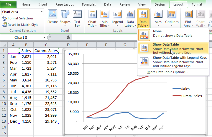
How-to Add a Line to an Excel Chart Data Table and Not to the Excel Graph - Excel Dashboard ...

How do you label data points in Excel? - profitclaims.com Right click the data series in the chart, and select Add Data Labels > Add Data Labels from the context menu to add data labels. 2. Click any data label to select all data labels, and then click the specified data label to select it only in the chart. 3.

How to change date format in axis of chart/Pivotchart in Excel?

How to change data point label color of a Waterfall chart? The following code snippet shows how to change data point label color of a Waterfall chart. Using excelEngine As ExcelEngine = New ExcelEngine () Dim application As IApplication = excelEngine. Excel application.

Chart's Data Series in Excel - Easy Excel Tutorial

How to Format Number to Millions in Excel (6 Ways) First, select the cell where we want to change the format in normal numbers to numbers in million. Cell D5 contains the original number. And we want to see the formatted number in cell E5. Second, to get the number in million units, we can use the formula. =D5/1000000 Simply divide the number by 1000000, as we know that million is equal to 1000000.

Target vs Actual Chart in Excel - Analytics Tuts

Excel Line Column Chart With 2 Axes On the Ribbon, click the Layout tab, under Chart Tools At the left end of the Ribbon, in the Current Selection group, click the drop down arrow Click Series "Cases" to select that series. To change a series chart type: In the chart, right-click on one of the selected Cases columns. In the shortcut menu that appears, click Change Series Chart Type

Share :